在R內實踐嶺回歸 (Doing Ridge regression in R Statistical software)

    如上次的百分位數回歸的一節所說, 作線性回歸的基本要求是LINE, 其中I(數據獨立性)和N(數據呈正態分佈)是較難符合要求的...
    不符合N時, 可試用百分位數回歸方法解決; 而不符合I時, 可試用嶺(岭)回歸方法!
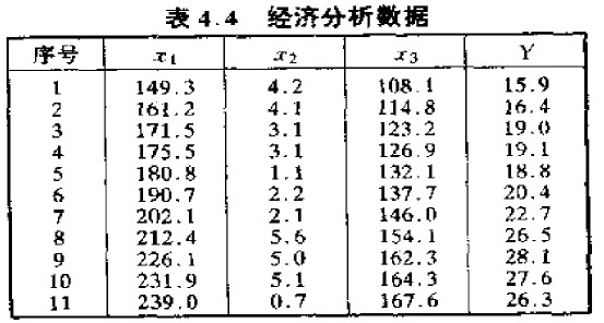
    為方便驗證是操作的正確性, 現引用高惠璇老師在《實用統計方法與SAS系統》P100-103例子作為對照! 好! 現在開始...
有這樣的一個數據:


#在R軟件內輸入並合成數據集d452, x1:國內生產總值, x2:儲存量, x3:總消費量, y:進口總額
x1<-c(149.3,161.2,171.5,175.5,180.8,190.7,202.1,212.4,226.1,231.9,239.0)
x2<-c(4.2,4.1,3.1,3.1,1.1,2.2,2.1,5.6,5.0,5.1,0.7)
x3<-c(108.1,114.8,123.2,126.9,132.1,137.7,146.0,154.1,162.3,164.3,167.6)
y<-c(15.9,16.4,19.0,19.1,18.8,20.4,22.7,26.5,28.1,27.6,26.3)
d452<-data.frame(x1,x2,x3,y)
lm.1<-lm(y~.,data = d452) #試作普通的線性回歸分析
summary(lm.1)
#結果

Call: lm(formula = y ~ ., data = d452)

Residuals:
     Min       1Q   Median       3Q      Max 
-0.52367 -0.38953  0.05424  0.22644  0.78313 

Coefficients:
             Estimate Std. Error t value Pr(>|t|)    
(Intercept) -10.12799    1.21216  -8.355  6.9e-05 ***
x1           -0.05140    0.07028  -0.731 0.488344    
x2            0.58695    0.09462   6.203 0.000444 ***
x3            0.28685    0.10221   2.807 0.026277 *  
---
Signif. codes:  0 ‘***’ 0.001 ‘**’ 0.01 ‘*’ 0.05 ‘.’ 0.1 ‘ ’ 1

Residual standard error: 0.4889 on 7 degrees of freedom
Multiple R-squared:  0.9919, Adjusted R-squared:  0.9884 
F-statistic: 285.6 on 3 and 7 DF,  p-value: 1.112e-07

x1為負值,與現實世界不符合... 

library(car)
vif.1<-vif(lm.1)
vif.1
#結果

        x1         x2         x3 
185.997470   1.018909 186.110015 

x1及x3的VIF大於10,有多重共線性 

cor.1<-cor.test(x1,x3)
cor.1
#結果

 Pearson's product-moment correlation

data:  x1 and x3
t = 40.448, df = 9, p-value = 1.718e-11
alternative hypothesis: true correlation is not equal to 0
95 percent confidence interval:
 0.9890918 0.9993142
sample estimates:
      cor 
0.9972607

x1與x3的相關系數達0.997(p<0.01),有強烈的相關性 

#在這種情況下,線性回歸的結果受多重共線性影響,方差會變得很大(因合力問題)!

為使方差變小,得加入一個系數(lambda).但這個系數的最小取值得依賴於方程中的β和σ2.

系數的估計方法有:

1. 嶺跡圖

2. 方差膨脹因子法

3. 控制殘差平方和法

library(MASS) #嶺回歸法在MASS的統計包內---lm.ridge命令
lm.r1<-lm.ridge(y~.,data = d452,lambda = seq(0,0.5,0.01)) #lambda系數可用seq序列, 讓函數自已試
#結果

                          x1        x2        x3
0.00 -10.127988 -0.051396160 0.5869490 0.2868487
0.01  -9.861266 -0.020071030 0.5920564 0.2411973
0.02  -9.696169 -0.001390176 0.5948969 0.2139345
...
0.50  -8.466721  0.064243563 0.5832040 0.1140136

嶺跡圖, 與lm.ridge的列表對應

plot(lm.r1)
select(lm.r1)
#結果

modified HKB estimator is 0.006855363
modified L-W estimator is 0.01283802 
smallest value of GCV  at 0.01

被選出最小的lambda系數是0.01 

lm.r2<-lm.ridge(y~.,data = d452,lambda = 0.01)
lm.r2
#結果

                     x1          x2          x3 
-9.86126637 -0.02007103  0.59205639  0.24119727 

若以lambda系數為0.01再代入計算,則得嶺回歸方程為上.

lm.r3<-lm.ridge(y~.,data = d452,lambda = 0.02)
lm.r3#結果

                       x1           x2           x3 
-9.696168972 -0.001390176  0.594896865  0.213934536

若以該書的0.02代入嶺回歸公式,得上述結果!與書的結果不符合...

lm.r4<-lm.ridge(y~.,data = d452,lambda = 0.22)
lm.r4 

#結果

                     x1          x2          x3 
-8.92769761  0.05734309  0.59541713  0.12663337 

這才與書上的結果一致...